拉格朗日插值

knn回归模型的优点之一是模型很容易理解，通常不需要过多的调参就可以得到不错的性能，并且构建模型的速度通常很快。但是使用knn算法时，对数据进行预处理是很重要的，对特征很多的数据集、对于大多数特征值都为0的数据集，效果往往不是很好。

虽然k邻近算法很容易理解，但是由于预测速度慢，且不能处理具有很多特征的数据集，所以，在实践中往往不会用到。

%matplotlib inline

import sys
print("Python version:", sys.version)

import pandas as pd
print("pandas version:", pd.__version__)

import matplotlib
print("matplotlib version:", matplotlib.__version__)

import numpy as np
print("NumPy version:", np.__version__)

import scipy as sp
print("SciPy version:", sp.__version__)

import IPython
print("IPython version:", IPython.__version__)

import sklearn
print("scikit-learn version:", sklearn.__version__)

import imblearn
print("imbanlced-learn version:",imblearn.__version__)

Python version: 3.7.1 (default, Dec 10 2018, 22:54:23) [MSC v.1915 64 bit (AMD64)]
pandas version: 0.23.4
matplotlib version: 3.0.2
NumPy version: 1.19.2
SciPy version: 1.6.2
IPython version: 7.2.0
scikit-learn version: 0.24.1
imbanlced-learn version: 0.8.0

import pandas as pd #导入数据分析库Pandas
import numpy as np
import matplotlib.pyplot as plt
import matplotlib

#指定默认字体
#matplotlib.rcParams['font.sans-serif'] = ['SimHei']
#matplotlib.rcParams['font.family']='sans-serif'
#matplotlib.rcParams['font.size']=14

plt.rc('figure', figsize=(10, 10))

font_options={'sans-serif':'SimHei','family':'sans-serif','weight':'bold','size':20}
plt.rc('font',**font_options)


#plt.style.use('ggplot') # ggplot是其中一种预设样式,会使用R的同学应该非常熟悉

#print(plt.style.available) # 查看所有预设样式
#from scipy.interpolate import lagrange #导入拉格朗日插值函数

inputfile = '../data/missing_data.xls' #输入数据路径,需要使用Excel格式；
outputfile = '../tmp/missing_data_processed.xls' #输出数据路径,需要使用Excel格式

data = pd.read_excel(inputfile, header=None) #读入数据

data

	0	1	2
0	235.8333	324.0343	478.3231
1	236.2708	325.6379	515.4564
2	238.0521	328.0897	517.0909
3	235.9063	NaN	514.8900
4	236.7604	268.8324	NaN
5	NaN	404.0480	486.0912
6	237.4167	391.2652	516.2330
7	238.6563	380.8241	NaN
8	237.6042	388.0230	435.3508
9	238.0313	206.4349	487.6750
10	235.0729	NaN	NaN
11	235.5313	400.0787	660.2347
12	NaN	411.2069	621.2346
13	234.4688	395.2343	611.3408
14	235.5000	344.8221	643.0863
15	235.6354	385.6432	642.3482
16	234.5521	401.6234	NaN
17	236.0000	409.6489	602.9347
18	235.2396	416.8795	589.3457
19	235.4896	NaN	556.3452
20	236.9688	NaN	538.3470

#拉格朗日插值代码
md_data=data.interpolate()
md_data

	0	1	2
0	235.83330	324.03430	478.32310
1	236.27080	325.63790	515.45640
2	238.05210	328.08970	517.09090
3	235.90630	298.46105	514.89000
4	236.76040	268.83240	500.49060
5	237.08855	404.04800	486.09120
6	237.41670	391.26520	516.23300
7	238.65630	380.82410	475.79190
8	237.60420	388.02300	435.35080
9	238.03130	206.43490	487.67500
10	235.07290	303.25680	573.95485
11	235.53130	400.07870	660.23470
12	235.00005	411.20690	621.23460
13	234.46880	395.23430	611.34080
14	235.50000	344.82210	643.08630
15	235.63540	385.64320	642.34820
16	234.55210	401.62340	622.64145
17	236.00000	409.64890	602.93470
18	235.23960	416.87950	589.34570
19	235.48960	416.87950	556.34520
20	236.96880	416.87950	538.34700

#输出结果
md_data.to_excel(outputfile,header=None,index=False)

模型构建

观察数据

from mglearn import plot_helpers

#构建CART决策树模型
from sklearn.tree import DecisionTreeClassifier #导入决策树模型

import matplotlib.pyplot as plt

datafile = '../data/model.xls' #数据名
data = pd.read_excel(datafile) #读取数据，数据的前三列是特征，第四列是标签

#对各个指标一次统计
data.apply(pd.value_counts)

	电量趋势下降指标	线损指标	告警类指标	是否窃漏电
0	50	142.0	100.0	251.0
1	44	149.0	74.0	40.0
2	48	NaN	95.0	NaN
3	47	NaN	11.0	NaN
4	50	NaN	11.0	NaN
5	31	NaN	NaN	NaN
6	8	NaN	NaN	NaN
7	5	NaN	NaN	NaN
8	2	NaN	NaN	NaN
9	4	NaN	NaN	NaN
10	2	NaN	NaN	NaN

data.head()

	电量趋势下降指标	线损指标	告警类指标	是否窃漏电
0	4	1	1	1
1	4	0	4	1
2	2	1	1	1
3	9	0	0	0
4	3	1	0	0

data.iloc[:,3:4].head()

	是否窃漏电
0	1
1	1
2	1
3	0
4	0

data.describe()

	电量趋势下降指标	线损指标	告警类指标	是否窃漏电
count	291.000000	291.000000	291.000000	291.000000
mean	2.718213	0.512027	1.171821	0.137457
std	2.091768	0.500716	1.065783	0.344922
min	0.000000	0.000000	0.000000	0.000000
25%	1.000000	0.000000	0.000000	0.000000
50%	3.000000	1.000000	1.000000	0.000000
75%	4.000000	1.000000	2.000000	0.000000
max	10.000000	1.000000	4.000000	1.000000

list(data.columns)
data.sum()

电量趋势下降指标    791
线损指标        149
告警类指标       341
是否窃漏电        40
dtype: int64

data[data.columns[3]].value_counts()

0    251
1     40
Name: 是否窃漏电, dtype: int64

data_group=data.groupby(list(data.columns)[3])
data_group.count()

	电量趋势下降指标	线损指标	告警类指标
是否窃漏电
0	251	251	251
1	40	40	40

Basic Plotting: plot See the cookbook for some advanced strategies

The plot method on Series and DataFrame is just a simple wrapper around plt.plot():

df.plot(kind='line') is equivalent to df.plot.line()

Other Plots The kind keyword argument of plot() accepts a handful of values for plots other than the default Line plot. These include:

‘bar’ or ‘barh’ for bar plots ‘hist’ for histogram ‘box’ for boxplot ‘kde’ or ‘density’ for density plots ‘area’ for area plots ‘scatter’ for scatter plots ‘hexbin’ for hexagonal bin plots ‘pie’ for pie plots In addition to these kind s, there are the DataFrame.hist(), and DataFrame.boxplot() methods, which use a separate interface.

Finally, there are several plotting functions in pandas.tools.plotting that take a Series or DataFrame as an argument. These include

Scatter Matrix Andrews Curves Parallel Coordinates Lag Plot Autocorrelation Plot Bootstrap Plot RadViz Plots may also be adorned with errorbars or tables.

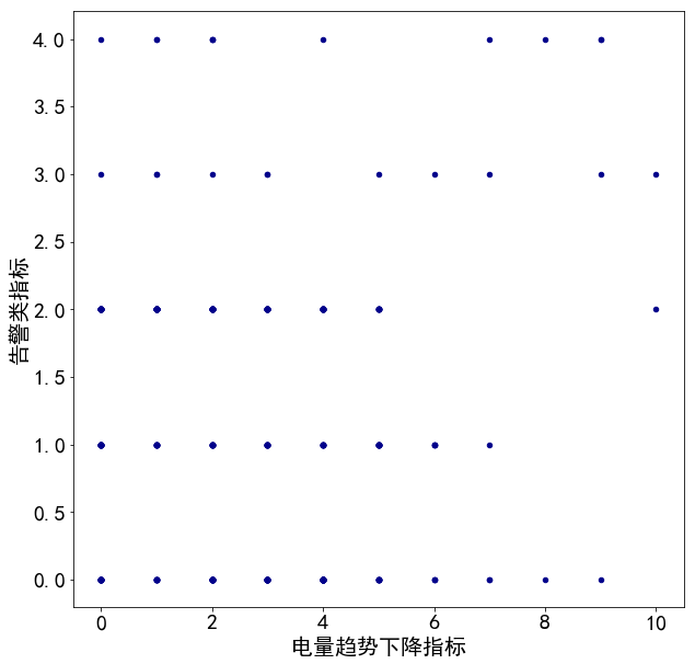
#data.plot.scatter(x='电量趋势下降指标',y='是否窃漏电',c='DarkBlue')
data.plot.scatter(x=list(data.columns)[0],y=list(data.columns)[2],c='DarkBlue')

<matplotlib.axes._subplots.AxesSubplot at 0x16bd2ca00b8>

png

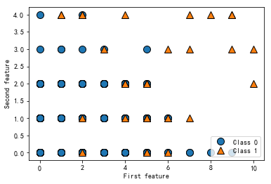
# plot dataset
plot_helpers.discrete_scatter(data.iloc[1:, 0], data.iloc[1:, 2], data.iloc[1:,3])
plt.legend(["Class 0", "Class 1"], loc=4)
plt.xlabel("First feature")
plt.ylabel("Second feature")
print("data[:,:3]].shape:", data.iloc[1:,:3].shape)

data[:,:3]].shape: (290, 3)

png

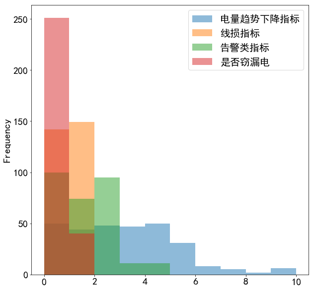
data.plot(kind='hist',alpha=0.5)#与data.plot.hist(alpha=05)造价

<matplotlib.axes._subplots.AxesSubplot at 0x1d52da54c18>

png

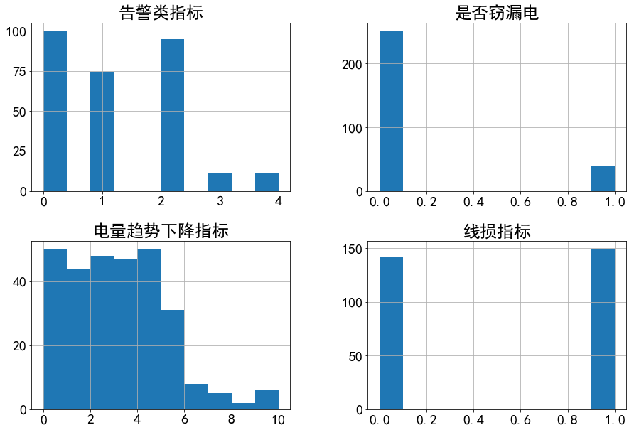
data.hist(figsize=(15,10))#分开绘图

array([[<matplotlib.axes._subplots.AxesSubplot object at 0x000001D52CFB8A90>,
        <matplotlib.axes._subplots.AxesSubplot object at 0x000001D52DB4A4E0>],
       [<matplotlib.axes._subplots.AxesSubplot object at 0x000001D52E06F978>,
        <matplotlib.axes._subplots.AxesSubplot object at 0x000001D52E092EB8>]],
      dtype=object)

png

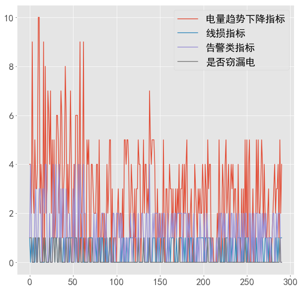
data.plot()

<matplotlib.axes._subplots.AxesSubplot at 0x2148b9d9160>

png

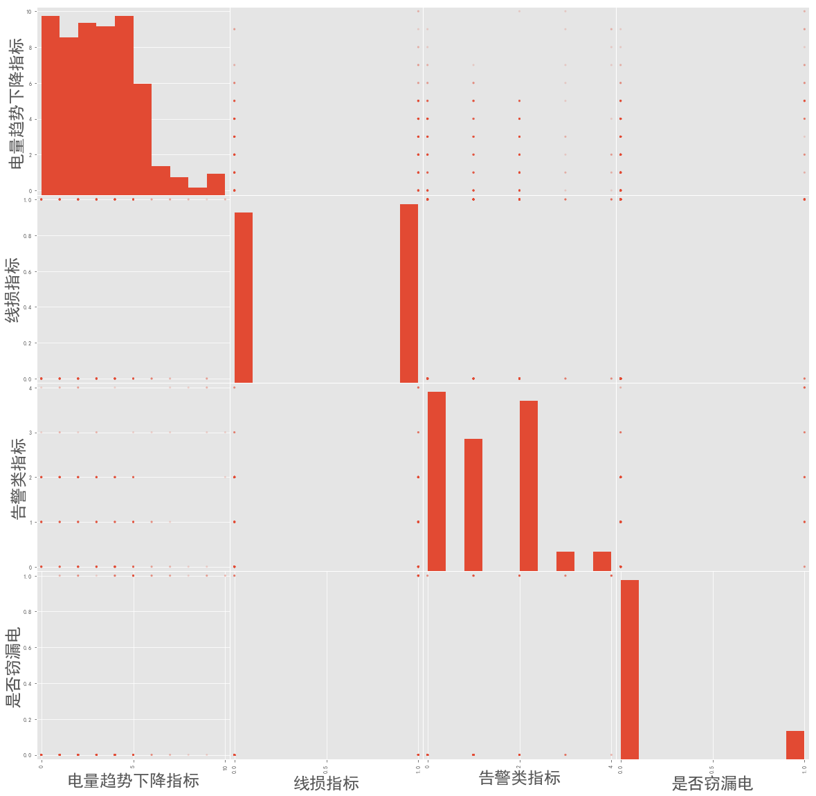
pd.plotting.scatter_matrix(data,figsize=(20,20),alpha=0.2)

array([[<matplotlib.axes._subplots.AxesSubplot object at 0x0000021489E34C50>,
        <matplotlib.axes._subplots.AxesSubplot object at 0x0000021489EADDA0>,
        <matplotlib.axes._subplots.AxesSubplot object at 0x000002148B5BF198>,
        <matplotlib.axes._subplots.AxesSubplot object at 0x000002148B5E66D8>],
       [<matplotlib.axes._subplots.AxesSubplot object at 0x000002148B60DC50>,
        <matplotlib.axes._subplots.AxesSubplot object at 0x000002148B63F208>,
        <matplotlib.axes._subplots.AxesSubplot object at 0x000002148B667780>,
        <matplotlib.axes._subplots.AxesSubplot object at 0x000002148B690D30>],
       [<matplotlib.axes._subplots.AxesSubplot object at 0x000002148B690D68>,
        <matplotlib.axes._subplots.AxesSubplot object at 0x000002148B6E8828>,
        <matplotlib.axes._subplots.AxesSubplot object at 0x000002148B712DA0>,
        <matplotlib.axes._subplots.AxesSubplot object at 0x000002148B743358>],
       [<matplotlib.axes._subplots.AxesSubplot object at 0x000002148B7698D0>,
        <matplotlib.axes._subplots.AxesSubplot object at 0x000002148B792E48>,
        <matplotlib.axes._subplots.AxesSubplot object at 0x000002148B7C2400>,
        <matplotlib.axes._subplots.AxesSubplot object at 0x000002148B7EA978>]],
      dtype=object)

png

构建KNN模型

#data[[list(data.columns)[0],list(data.columns)[2]]]=data[[list(data.columns)[0],list(data.columns)[2]]].astype(str)

data_dummies=pd.get_dummies(data,columns=[list(data.columns)[0],list(data.columns)[2]])

data_dummies

	线损指标	是否窃漏电	电量趋势下降指标_0	电量趋势下降指标_1	电量趋势下降指标_2	电量趋势下降指标_3	电量趋势下降指标_4	电量趋势下降指标_5	电量趋势下降指标_6	电量趋势下降指标_7	电量趋势下降指标_8	电量趋势下降指标_9	电量趋势下降指标_10	告警类指标_0	告警类指标_1	告警类指标_2	告警类指标_3	告警类指标_4
0	1	1	0	0	0	0	1	0	0	0	0	0	0	0	1	0	0	0
1	0	1	0	0	0	0	1	0	0	0	0	0	0	0	0	0	0	1
2	1	1	0	0	1	0	0	0	0	0	0	0	0	0	1	0	0	0
3	0	0	0	0	0	0	0	0	0	0	0	1	0	1	0	0	0	0
4	1	0	0	0	0	1	0	0	0	0	0	0	0	1	0	0	0	0
...	...	...	...	...	...	...	...	...	...	...	...	...	...	...	...	...	...	...
286	1	0	0	0	0	0	1	0	0	0	0	0	0	0	0	1	0	0
287	0	0	0	1	0	0	0	0	0	0	0	0	0	0	0	1	0	0
288	1	1	0	0	0	0	0	1	0	0	0	0	0	0	0	1	0	0
289	1	0	0	0	1	0	0	0	0	0	0	0	0	1	0	0	0	0
290	1	0	0	0	0	0	1	0	0	0	0	0	0	1	0	0	0	0

291 rows × 18 columns

data_dummies_cols=list(data_dummies.columns)
first_col=data_dummies_cols.pop(0)
second_col=data_dummies_cols.pop(0)

data_dummies_cols=data_dummies_cols+[first_col,second_col]

data_dummies_cols

['电量趋势下降指标_0',
 '电量趋势下降指标_1',
 '电量趋势下降指标_2',
 '电量趋势下降指标_3',
 '电量趋势下降指标_4',
 '电量趋势下降指标_5',
 '电量趋势下降指标_6',
 '电量趋势下降指标_7',
 '电量趋势下降指标_8',
 '电量趋势下降指标_9',
 '电量趋势下降指标_10',
 '告警类指标_0',
 '告警类指标_1',
 '告警类指标_2',
 '告警类指标_3',
 '告警类指标_4',
 '线损指标',
 '是否窃漏电']

data_dummies=data_dummies[data_dummies_cols]#.astype(int)
data_dummies

	电量趋势下降指标_0	电量趋势下降指标_1	电量趋势下降指标_2	电量趋势下降指标_3	电量趋势下降指标_4	电量趋势下降指标_5	电量趋势下降指标_6	电量趋势下降指标_7	电量趋势下降指标_8	电量趋势下降指标_9	电量趋势下降指标_10	告警类指标_0	告警类指标_1	告警类指标_2	告警类指标_3	告警类指标_4	线损指标	是否窃漏电
0	0	0	0	0	1	0	0	0	0	0	0	0	1	0	0	0	1	1
1	0	0	0	0	1	0	0	0	0	0	0	0	0	0	0	1	0	1
2	0	0	1	0	0	0	0	0	0	0	0	0	1	0	0	0	1	1
3	0	0	0	0	0	0	0	0	0	1	0	1	0	0	0	0	0	0
4	0	0	0	1	0	0	0	0	0	0	0	1	0	0	0	0	1	0
...	...	...	...	...	...	...	...	...	...	...	...	...	...	...	...	...	...	...
286	0	0	0	0	1	0	0	0	0	0	0	0	0	1	0	0	1	0
287	0	1	0	0	0	0	0	0	0	0	0	0	0	1	0	0	0	0
288	0	0	0	0	0	1	0	0	0	0	0	0	0	1	0	0	1	1
289	0	0	1	0	0	0	0	0	0	0	0	1	0	0	0	0	1	0
290	0	0	0	0	1	0	0	0	0	0	0	1	0	0	0	0	1	0

291 rows × 18 columns

data_dummies = data_dummies.values #将表格转换为矩阵
data_dummies

array([[0, 0, 0, ..., 0, 1, 1],
       [0, 0, 0, ..., 1, 0, 1],
       [0, 0, 1, ..., 0, 1, 1],
       ...,
       [0, 0, 0, ..., 0, 1, 1],
       [0, 0, 1, ..., 0, 1, 0],
       [0, 0, 0, ..., 0, 1, 0]], dtype=int64)

data_dummies[:,-1]

array([0, 1, 0, 0, 0, 0, 0, 0, 0, 0, 0, 0, 0, 0, 0, 0, 0, 0, 1, 1, 0, 0,
       0, 0, 0, 0, 0, 1, 0, 0, 1, 0, 0, 0, 1, 0, 0, 0, 0, 0, 0, 0, 0, 0,
       0, 0, 0, 0, 0, 0, 0, 0, 1, 0, 0, 0, 1, 0, 1, 0, 0, 0, 1, 0, 0, 0,
       0, 0, 0, 0, 0, 0, 0, 0, 0, 0, 0, 0, 0, 0, 0, 0, 0, 0, 0, 0, 0, 0,
       0, 0, 0, 0, 0, 0, 0, 0, 0, 0, 0, 0, 0, 0, 0, 0, 0, 0, 0, 0, 0, 0,
       0, 0, 0, 0, 0, 0, 0, 0, 0, 0, 0, 0, 0, 0, 0, 0, 0, 0, 0, 0, 0, 0,
       0, 0, 0, 0, 0, 0, 1, 0, 0, 0, 0, 0, 0, 0, 0, 0, 0, 0, 0, 0, 0, 0,
       0, 0, 0, 0, 0, 0, 0, 0, 0, 0, 0, 0, 0, 0, 0, 0, 0, 0, 0, 0, 0, 0,
       0, 0, 0, 0, 0, 0, 0, 0, 0, 0, 0, 0, 0, 0, 0, 0, 0, 0, 0, 0, 0, 0,
       0, 0, 0, 0, 0, 0, 0, 0, 0, 0, 0, 0, 0, 0, 0, 0, 0, 0, 0, 0, 0, 0,
       0, 0, 0, 0, 0, 0, 0, 0, 0, 0, 0, 0, 0, 0, 0, 0, 0, 0, 0, 0, 0, 0,
       0, 0, 0, 0, 0, 0, 0, 0, 0, 0, 0, 0, 0, 0, 0, 0, 0, 0, 0, 0, 0, 0,
       0, 0, 0, 0, 0, 0, 0, 0, 0, 0, 0, 0, 0, 0, 0, 0, 0, 0, 0, 0, 0, 0,
       0, 0, 0, 0, 0], dtype=int64)

data_dummies.shape[1]

from sklearn.model_selection import train_test_split

#train_test_split Parameters
#test_size : float, int or None, optional (default=0.25)
#shuffle : boolean, optional (default=True)
#X_train,X_test,y_train,y_test=train_test_split(data_dummies[:,:data_dummies.shape[1]-1],data_dummies[:,-1],random_state=0)
X_train,X_test,y_train,y_test=train_test_split(data_dummies[:,:-1],data_dummies[:,-1],random_state=60)

X_train

array([[1, 0, 0, ..., 0, 0, 0],
       [1, 0, 0, ..., 0, 0, 0],
       [0, 0, 0, ..., 0, 0, 0],
       ...,
       [0, 1, 0, ..., 0, 0, 0],
       [0, 1, 0, ..., 0, 0, 0],
       [0, 0, 0, ..., 0, 1, 0]], dtype=int64)

y_train

array([0, 0, 0, 0, 0, 0, 0, 0, 0, 0, 0, 0, 0, 1, 0, 1, 0, 0, 0, 0, 0, 0,
       0, 0, 0, 0, 0, 0, 0, 0, 0, 0, 0, 0, 0, 1, 0, 0, 0, 0, 1, 0, 0, 0,
       0, 0, 0, 0, 0, 0, 1, 0, 0, 0, 0, 0, 0, 0, 0, 0, 0, 0, 0, 0, 0, 1,
       0, 1, 0, 0, 0, 0, 0, 0, 0, 1, 0, 1, 0, 0, 0, 0, 1, 0, 1, 0, 0, 0,
       0, 0, 0, 0, 0, 1, 0, 0, 0, 0, 0, 0, 0, 1, 0, 0, 0, 0, 0, 0, 0, 1,
       0, 0, 1, 0, 0, 1, 0, 0, 0, 0, 0, 0, 0, 0, 1, 0, 1, 0, 0, 0, 0, 0,
       0, 0, 1, 0, 0, 0, 1, 1, 0, 0, 0, 0, 0, 0, 0, 0, 0, 0, 0, 0, 1, 0,
       0, 0, 0, 0, 0, 1, 0, 0, 0, 1, 0, 0, 0, 0, 0, 0, 0, 1, 0, 0, 0, 1,
       1, 0, 0, 0, 0, 0, 0, 0, 1, 0, 0, 0, 0, 0, 0, 0, 0, 0, 0, 0, 0, 1,
       0, 0, 0, 0, 0, 0, 0, 0, 0, 0, 0, 0, 0, 0, 0, 0, 0, 0, 1, 1],
      dtype=int64)

X_test

array([[0, 0, 0, ..., 1, 0, 0],
       [0, 0, 1, ..., 0, 0, 0],
       [0, 0, 0, ..., 0, 0, 0],
       ...,
       [0, 0, 0, ..., 0, 1, 0],
       [1, 0, 0, ..., 0, 1, 0],
       [1, 0, 0, ..., 1, 0, 0]], dtype=int64)

print("X_train shape:", X_train.shape)
print("y_train shape:", y_train.shape)
print("y_test shape:", y_test.shape)

X_train shape: (218, 17)
y_train shape: (218,)
y_test shape: (73,)

Logistic回归从根本上解决因变量要不是连续变量怎么办的问题。自变量既可以是连续的，也可以是分类的。然后通过logistic回归分析，可以得到自变量的权重，从而可以大致了解到底哪些因素是胃癌的危险因素。同时根据该权值可以根据危险因素预测一个人患癌症的可能性。 Logistic回归模型的适用条件 1 因变量为二分类的分类变量或某事件的发生率，并且是数值型变量。但是需要注意，重复计数现象指标不适用于Logistic回归。 2 残差和因变量都要服从二项分布。二项分布对应的是分类变量，所以不是正态分布，进而不是用最小二乘法，而是最大似然法来解决方程估计和检验问题。 3 自变量和Logistic概率是线性关系 4 各观测对象间相互独立。

from sklearn.linear_model import LogisticRegression

import numpy as np y = [0,0,0,0,0,0,0,0,1,1,1,1,1,1,2,2] #标签值，一共16个样本 a = np.bincount(y) # array([8, 6, 2], dtype=int64) 计算每个类别的样本数量 aa = 1/a #倒数 array([0.125 , 0.16666667, 0.5 ]) print(aa)

from sklearn.utils.class_weight import compute_class_weight class_weight = ‘balanced’ classes = np.array([0, 1, 2]) #标签类别 weight = compute_class_weight(class_weight, classes, y) print(weight) # [0.66666667 0.88888889 2.66666667]

print(0.666666678) #5.33333336 print(0.888888896) #5.33333334 print(2.66666667*2) #5.33333334 #这三个值非常接近 ‘balanced’计算出来的结果很均衡，使得惩罚项和样本量对应

#由于原始数据不均衡，引入class_weight='balanced'
lg=LogisticRegression(C=1,solver='lbfgs',class_weight='balanced')

lg.fit(X_train,y_train)

LogisticRegression(C=1, class_weight='balanced')

#模型学到的自变量系数
lg.coef_

array([[-1.8982079 , -1.50770935, -0.30930785, -1.54120769,  0.01474898,
         1.56566034,  1.02127487,  0.8846096 , -0.03445342,  0.95543708,
         0.84902324, -1.79004659, -0.83005007, -0.50817373,  1.13049358,
         1.99764472,  1.79664114]])

评估模型

y_pred=lg.predict(X_test)
y_pred

array([0, 0, 0, 0, 0, 1, 0, 0, 1, 0, 1, 0, 0, 0, 1, 0, 0, 1, 0, 0, 1, 1,
       0, 0, 0, 0, 0, 0, 0, 0, 0, 0, 1, 0, 0, 0, 0, 1, 0, 1, 0, 0, 1, 0,
       0, 1, 0, 0, 0, 1, 0, 0, 0, 1, 0, 0, 0, 0, 0, 1, 0, 1, 0, 0, 0, 0,
       0, 1, 0, 1, 0, 0, 1], dtype=int64)

#Accuracy=(TP+TN)/(TP+TN+FP+FN)，正确识别率=(60+8)/(60+8+3+2)
lg.score(X_test,y_test)

0.863013698630137

from sklearn.metrics import confusion_matrix
confusion=confusion_matrix(y_test,y_pred)

y_test.sum()

y_test.size

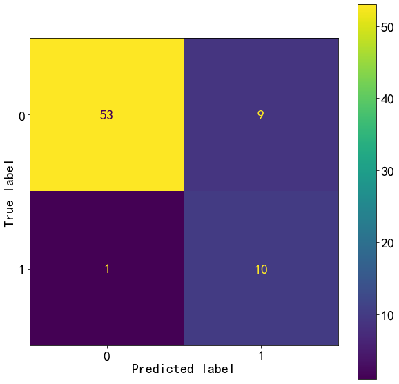
confusion

array([[53,  9],
       [ 1, 10]], dtype=int64)

from sklearn.metrics import plot_confusion_matrix
plot_confusion_matrix(lg,X_test,y_test)

<sklearn.metrics._plot.confusion_matrix.ConfusionMatrixDisplay at 0x2457c5a5748>

png

from sklearn.metrics import f1_score

test_score=f1_score(y_test,y_pred)

test_score

0.6666666666666666

from sklearn.metrics import classification_report

test_report=classification_report(y_test,y_pred,target_names=["0","1"])

#precision=TP/(TP+FP),如{1}：8/(8+2),{0}:60/(60+3)。FP假正例，为预测正确实际错误
#recall=TP/(TP+FN)，{1}：8/（8+3),{0}:60/(60+2)。FN假反例，预测错误实际正确
#这个项目1的recall非常重要，数据不平衡，因此引入class_weight='balanced'
print(test_report)

              precision    recall  f1-score   support

           0       0.98      0.85      0.91        62
           1       0.53      0.91      0.67        11

    accuracy                           0.86        73
   macro avg       0.75      0.88      0.79        73
weighted avg       0.91      0.86      0.88        73

y_pred_lower_threshold=lg.decision_function(X_test)>-0.5

test_report_lower_theshold=classification_report(y_test,y_pred_lower_threshold)
print(test_report_lower_theshold)

---------------------------------------------------------------------------

NameError                                 Traceback (most recent call last)

<ipython-input-29-99dfdd4c5dbd> in <module>
----> 1 test_report_lower_theshold=classification_report(y_test,y_pred_lower_threshold)
      2 print(test_report_lower_theshold)


NameError: name 'classification_report' is not defined

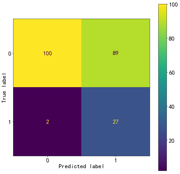
y_train_pred=lg.predict(X_train)

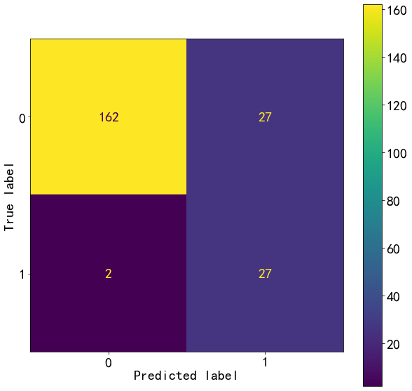
confusion_train=confusion_matrix(y_train,y_train_pred)

confusion_train

array([[162,  27],
       [  2,  27]], dtype=int64)

plot_confusion_matrix(lg,X_train,y_train)

<sklearn.metrics._plot.confusion_matrix.ConfusionMatrixDisplay at 0x2457cc850c8>

png

print(classification_report(y_train,y_train_pred,target_names=['0','1']))

              precision    recall  f1-score   support

           0       0.99      0.86      0.92       189
           1       0.50      0.93      0.65        29

    accuracy                           0.87       218
   macro avg       0.74      0.89      0.78       218
weighted avg       0.92      0.87      0.88       218

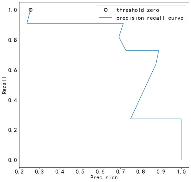
准确率-召回率曲线

from sklearn.metrics import precision_recall_curve

#predict_proba:  模型预测输入样本属于每种类别的概率，概率和为1，每个位置的概率分别对应classes_中对应位置的类别标签。knn.class_=[0,1]
lg.predict_proba(X_test)[:,1]

array([0.04807361, 0.0129165 , 0.01835642, 0.22136398, 0.23341758,
       0.86809927, 0.27874242, 0.08141368, 0.73891599, 0.06023652,
       0.50232206, 0.29582958, 0.23341758, 0.19533512, 0.58204273,
       0.36619901, 0.18763114, 0.86809927, 0.34827022, 0.01835642,
       0.88576147, 0.86809927, 0.29582958, 0.24205981, 0.24205981,
       0.0129165 , 0.29582958, 0.18763114, 0.28889944, 0.1013232 ,
       0.06513878, 0.06023652, 0.94464191, 0.07312772, 0.34827022,
       0.01835642, 0.06312835, 0.65818615, 0.22136398, 0.90079889,
       0.08141368, 0.34827022, 0.65818615, 0.06312835, 0.14339758,
       0.58204273, 0.0129165 , 0.06312835, 0.24205981, 0.86809927,
       0.06513878, 0.03304592, 0.27874242, 0.79647369, 0.29582958,
       0.06312835, 0.19516898, 0.28889944, 0.34827022, 0.58257308,
       0.34827022, 0.98372519, 0.18796373, 0.08141368, 0.1013232 ,
       0.18763114, 0.08141368, 0.71590931, 0.03304592, 0.52188984,
       0.06513878, 0.28889944, 0.50232206])

precision,recall,thresholds=precision_recall_curve(y_test,lg.predict_proba(X_test)[:,1])

thresholds

array([0.19516898, 0.19533512, 0.22136398, 0.23341758, 0.24205981,
       0.27874242, 0.28889944, 0.29582958, 0.34827022, 0.36619901,
       0.50232206, 0.52188984, 0.58204273, 0.58257308, 0.65818615,
       0.71590931, 0.73891599, 0.79647369, 0.86809927, 0.88576147,
       0.90079889, 0.94464191, 0.98372519])

# find threshold closest to zero
close_zero = np.argmin(np.abs(thresholds))
plt.plot(precision[close_zero], recall[close_zero], 'o', markersize=10,
         label="threshold zero", fillstyle="none", c='k', mew=2)

plt.plot(precision, recall, label="precision recall curve")
plt.xlabel("Precision")
plt.ylabel("Recall")
plt.legend(loc="best")

<matplotlib.legend.Legend at 0x2457c51a508>

png

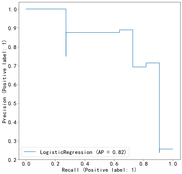
from sklearn.metrics import plot_precision_recall_curve
plot_precision_recall_curve(lg,X_test,y_test)

<sklearn.metrics._plot.precision_recall_curve.PrecisionRecallDisplay at 0x2457c7dc6c8>

png

#from sklearn.metrics import plot_confusion_matrix
from sklearn.metrics import plot_confusion_matrix

from sklearn.metrics import average_precision_score

ap_clf=average_precision_score(y_test,lg.predict_proba(X_test)[:,1])
ap_clf

0.8228451135427879

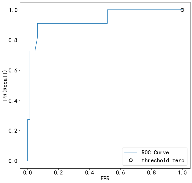
from sklearn.metrics import roc_curve

fpr,tpr,thresholds=roc_curve(y_test,lg.predict_proba(X_test)[:,1])
plt.plot(fpr,tpr,label="ROC Curve")
plt.xlabel('FPR')
plt.ylabel('TPR(Recall)')
#找到最接近于0的阈值
close_zero=np.argmin(np.abs(thresholds))
plt.plot(fpr[close_zero],tpr[close_zero],'o',markersize=10,label='threshold zero',fillstyle='none',c='k',mew=2)
plt.legend(loc=4)

<matplotlib.legend.Legend at 0x2457c2db708>

png

from sklearn.metrics import plot_roc_curve
plot_roc_curve(lg,X_test,y_test)

<sklearn.metrics._plot.roc_curve.RocCurveDisplay at 0x2457ca46688>

png

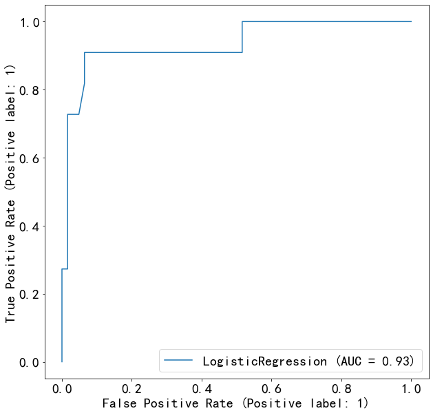
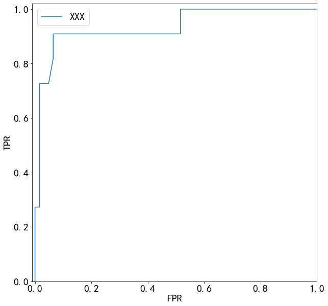
from sklearn.metrics import roc_auc_score

auc=roc_auc_score(y_test,lg.predict_proba(X_test)[:,1])
print('AUC={:.2f}'.format(auc))
fpr,tpr,_=roc_curve(y_test,lg.predict_proba(X_test)[:,1])
plt.plot(fpr,tpr,label='XXX')
plt.xlabel('FPR')
plt.ylabel('TPR')
plt.xlim(-0.01,1)
plt.ylim(0,1.02)
plt.legend(loc='best')

AUC=0.93

<matplotlib.legend.Legend at 0x2457ec5b708>

png

from sklearn.model_selection import GridSearchCV
from sklearn.linear_model import LogisticRegression
param_grid=[{'penalty':['l2'],'class_weight':['balanced',None],'solver':['sag','lbfgs','newton-cg']},
           {'penalty':['l1'],'class_weight':['balanced',None],'solver':['saga']},
           {'penalty':['l1','l2'],'class_weight':['balanced',None],'solver':['liblinear']}]
grid_search=GridSearchCV(LogisticRegression(max_iter=1000),param_grid,cv=5,scoring='recall')

grid_search.fit(X_train,y_train)

C:\Users\SF\Anaconda3\lib\site-packages\sklearn\linear_model\_sag.py:329: ConvergenceWarning: The max_iter was reached which means the coef_ did not converge
  "the coef_ did not converge", ConvergenceWarning)
C:\Users\SF\Anaconda3\lib\site-packages\sklearn\linear_model\_sag.py:329: ConvergenceWarning: The max_iter was reached which means the coef_ did not converge
  "the coef_ did not converge", ConvergenceWarning)
C:\Users\SF\Anaconda3\lib\site-packages\sklearn\linear_model\_sag.py:329: ConvergenceWarning: The max_iter was reached which means the coef_ did not converge
  "the coef_ did not converge", ConvergenceWarning)
C:\Users\SF\Anaconda3\lib\site-packages\sklearn\linear_model\_sag.py:329: ConvergenceWarning: The max_iter was reached which means the coef_ did not converge
  "the coef_ did not converge", ConvergenceWarning)
C:\Users\SF\Anaconda3\lib\site-packages\sklearn\linear_model\_sag.py:329: ConvergenceWarning: The max_iter was reached which means the coef_ did not converge
  "the coef_ did not converge", ConvergenceWarning)





GridSearchCV(cv=5, estimator=LogisticRegression(max_iter=10000),
             param_grid=[{'class_weight': ['balanced', None], 'penalty': ['l2'],
                          'solver': ['sag', 'lbfgs', 'newton-cg']},
                         {'class_weight': ['balanced', None], 'penalty': ['l1'],
                          'solver': ['saga']},
                         {'class_weight': ['balanced', None],
                          'penalty': ['l1', 'l2'], 'solver': ['liblinear']}],
             scoring='recall')

grid_search.score(X_test,y_test)

0.9090909090909091

grid_search.best_estimator_

LogisticRegression(class_weight='balanced', max_iter=10000, solver='liblinear')

grid_search.best_params_

{'class_weight': 'balanced', 'penalty': 'l2', 'solver': 'liblinear'}

results=pd.DataFrame(grid_search.cv_results_)
results.head()

	mean_fit_time	std_fit_time	mean_score_time	std_score_time	param_class_weight	param_penalty	param_solver	params	split0_test_score	split1_test_score	split2_test_score	split3_test_score	split4_test_score	mean_test_score	std_test_score	rank_test_score
0	0.006589	0.002055	0.000791	3.956447e-04	balanced	l2	sag	{'class_weight': 'balanced', 'penalty': 'l2', ...	0.833333	0.833333	0.833333	0.8	0.666667	0.793333	0.064636	2
1	0.004988	0.000630	0.000796	3.981196e-04	balanced	l2	lbfgs	{'class_weight': 'balanced', 'penalty': 'l2', ...	0.833333	0.833333	0.833333	0.8	0.666667	0.793333	0.064636	2
2	0.004792	0.000402	0.000998	1.907349e-07	balanced	l2	newton-cg	{'class_weight': 'balanced', 'penalty': 'l2', ...	0.833333	0.833333	0.833333	0.8	0.666667	0.793333	0.064636	2
3	0.001591	0.000496	0.000598	4.885776e-04	None	l2	sag	{'class_weight': None, 'penalty': 'l2', 'solve...	0.166667	0.666667	0.333333	0.0	0.333333	0.300000	0.221108	8
4	0.003790	0.000399	0.000598	4.886555e-04	None	l2	lbfgs	{'class_weight': None, 'penalty': 'l2', 'solve...	0.166667	0.666667	0.333333	0.0	0.333333	0.300000	0.221108	8

m_best=grid_search.best_estimator_
from sklearn.metrics import precision_score
y_pred=m_best.predict(X_test)
precision_score(y_test,y_pred)

0.5263157894736842

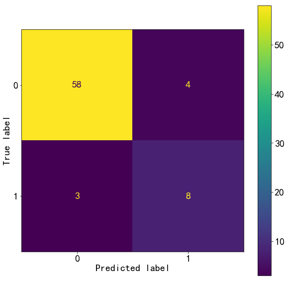
from sklearn.metrics import plot_confusion_matrix
plot_confusion_matrix(m_best,X_test,y_test)

<sklearn.metrics._plot.confusion_matrix.ConfusionMatrixDisplay at 0x2040cc2f198>

png

from sklearn.metrics import classification_report
test_report=classification_report(y_test,y_pred,target_names=["0","1"])
print(test_report)

              precision    recall  f1-score   support

           0       0.98      0.85      0.91        62
           1       0.53      0.91      0.67        11

    accuracy                           0.86        73
   macro avg       0.75      0.88      0.79        73
weighted avg       0.91      0.86      0.88        73

决策树：离散型数据1

data = data.values #将表格转换为矩阵
from sklearn.model_selection import train_test_split

#train_test_split Parameters
#test_size : float, int or None, optional (default=0.25)
#shuffle : boolean, optional (default=True)
X_train,X_test,y_train,y_test=train_test_split(data[:,:3],data[:,3],random_state=60)

from sklearn.model_selection import GridSearchCV
from sklearn.tree import DecisionTreeClassifier
param_grid=[{'criterion':['entropy'],'min_impurity_decrease':np.linspace(0,1,50)},
            {'criterion':['gini'],'min_impurity_decrease':np.linspace(0,0.5,50)},
             {'max_depth':range(2,11)},
             {'min_samples_split':range(2,30,2)}]
grid_search=GridSearchCV(DecisionTreeClassifier(),param_grid,cv=5,scoring='recall')

from sklearn.model_selection import GridSearchCV
from sklearn.tree import DecisionTreeClassifier
param_grid={'criterion':['gini','entropy'],'splitter':['best','random'],'max_depth':range(2,11),
            'min_samples_split':range(2,30,2),'min_samples_leaf':range(2,11)}

grid_search=GridSearchCV(DecisionTreeClassifier(random_state=0),param_grid,cv=5,scoring='recall')

grid_search.fit(X_train,y_train)

GridSearchCV(cv=5, estimator=DecisionTreeClassifier(random_state=0),
             param_grid={'criterion': ['gini', 'entropy'],
                         'max_depth': range(2, 11),
                         'min_samples_leaf': range(2, 11),
                         'min_samples_split': range(2, 30, 2),
                         'splitter': ['best', 'random']},
             scoring='recall')

grid_search.best_params_()

{'criterion': 'gini',
 'max_depth': 6,
 'min_samples_leaf': 2,
 'min_samples_split': 18,
 'splitter': 'random'}

grid_search.best_score_

0.7933333333333334

grid_search.best_estimator_

DecisionTreeClassifier(max_depth=6, min_samples_leaf=2, min_samples_split=18,
                       random_state=0, splitter='random')

m_best=grid_search.best_estimator_
from sklearn.metrics import precision_score
y_pred=m_best.predict(X_test)
precision_score(y_test,y_pred)

0.6666666666666666

m_best.score(X_train,y_train)

0.926605504587156

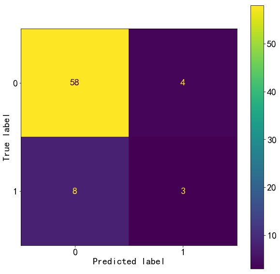
from sklearn.metrics import plot_confusion_matrix
plot_confusion_matrix(m_best,X_test,y_test)

<sklearn.metrics._plot.confusion_matrix.ConfusionMatrixDisplay at 0x2040d6b3e80>

png

from sklearn.metrics import classification_report
test_report=classification_report(y_test,y_pred,target_names=["0","1"])
print(test_report)

              precision    recall  f1-score   support

           0       0.95      0.94      0.94        62
           1       0.67      0.73      0.70        11

    accuracy                           0.90        73
   macro avg       0.81      0.83      0.82        73
weighted avg       0.91      0.90      0.91        73

imblearn,决策树

注意：对训练集和测试集都要重新采样。在重采样以减轻数据不平衡问题时，存在一个常见的陷阱，该陷阱为在将整个数据集拆分为训练集和测试集之前对整个数据集进行重采样。

这样的处理导致两个问题：

通过对整个数据集进行重新采样，训练集和测试集都可能得到平衡，而模型应该在自然不平衡的数据集上进行测试，以评估模型的潜在偏差。

重新采样过程可能会使用数据集中样本的信息来生成或选择一些样本。因此，我们可能会使用样本信息，这些信息以后将用作测试样本，这是典型的数据泄漏问题。 from imblearn.under_sampling import RandomUnderSampler 重采样的正确方法是使用Pipeline对训练集和测试集分别重新采样，这样可以避免任何数据泄漏。

data = data.values #将表格转换为矩阵
from sklearn.model_selection import train_test_split

#train_test_split Parameters
#test_size : float, int or None, optional (default=0.25)
#shuffle : boolean, optional (default=True)
X_train,X_test,y_train,y_test=train_test_split(data[:,:3],data[:,3],random_state=60)

from imblearn.pipeline import Pipeline
from imblearn.under_sampling import RandomUnderSampler
from sklearn.tree import DecisionTreeClassifier
pipe=Pipeline([('imblearn',RandomUnderSampler(random_state=0)),('clf',DecisionTreeClassifier(random_state=0))])

from sklearn.model_selection import GridSearchCV

param_grid={'clf__criterion':['gini','entropy'],'clf__splitter':['best','random'],'clf__max_depth':range(2,11),
            'clf__min_samples_split':range(2,30,2),'clf__min_samples_leaf':range(2,11)}

grid_search=GridSearchCV(pipe,param_grid,cv=5,scoring='recall')

grid_search.fit(X_train,y_train)

GridSearchCV(cv=5,
             estimator=Pipeline(steps=[('imblearn',
                                        RandomUnderSampler(random_state=0)),
                                       ('clf',
                                        DecisionTreeClassifier(random_state=0))]),
             param_grid={'clf__criterion': ['gini', 'entropy'],
                         'clf__max_depth': range(2, 11),
                         'clf__min_samples_leaf': range(2, 11),
                         'clf__min_samples_split': range(2, 30, 2),
                         'clf__splitter': ['best', 'random']},
             scoring='recall')

grid_search.best_params_()

---------------------------------------------------------------------------

TypeError                                 Traceback (most recent call last)

<ipython-input-16-522bf72df7ed> in <module>
----> 1 grid_search.best_params_()

TypeError: 'dict' object is not callable

grid_search.best_score_

0.8666666666666668

grid_search.best_estimator_

Pipeline(steps=[('imblearn', RandomUnderSampler(random_state=0)),
                ('clf',
                 DecisionTreeClassifier(max_depth=2, min_samples_leaf=2,
                                        random_state=0, splitter='random'))])

m_best=grid_search.best_estimator_
from sklearn.metrics import balanced_accuracy_score
y_test_pred=m_best.predict(X_test)
balanced_accuracy_score(y_test,y_pred)

0.7419354838709677

m_best.score(X_train,y_train)

0.5825688073394495

m_best.score(X_train,y_train)

0.5825688073394495

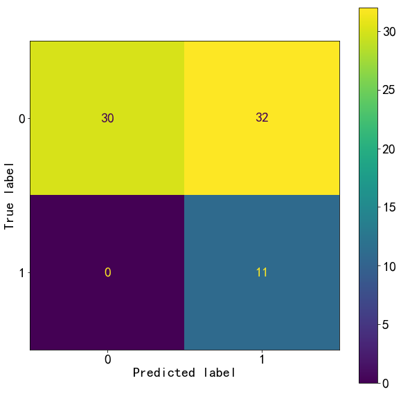
from sklearn.metrics import plot_confusion_matrix
plot_confusion_matrix(m_best,X_test,y_test)

<sklearn.metrics._plot.confusion_matrix.ConfusionMatrixDisplay at 0x1aef8921358>

png

from sklearn.metrics import classification_report
test_report=classification_report(y_test,y_test_pred,target_names=["0","1"])
print(test_report)

              precision    recall  f1-score   support

           0       1.00      0.48      0.65        62
           1       0.26      1.00      0.41        11

    accuracy                           0.56        73
   macro avg       0.63      0.74      0.53        73
weighted avg       0.89      0.56      0.62        73

plot_confusion_matrix(m_best,X_train,y_train)

<sklearn.metrics._plot.confusion_matrix.ConfusionMatrixDisplay at 0x1aef86ba2b0>

png

y_train_pred=m_best.predict(X_train)
train_report=classification_report(y_train,y_train_pred,target_names=["0","1"])
print(train_report)

              precision    recall  f1-score   support

           0       0.98      0.53      0.69       189
           1       0.23      0.93      0.37        29

    accuracy                           0.58       218
   macro avg       0.61      0.73      0.53       218
weighted avg       0.88      0.58      0.65       218

文档信息

本文作者：danielsywang
本文链接：https://danielsywang.github.io/2019/05/23/ml-prictice-classifier/
版权声明：自由转载-非商用-非衍生-保持署名（创意共享3.0许可证）

书生

电力窃漏电用户自动识别——分类算法分析比较

拉格朗日插值

模型构建

决策树：离散型数据1

imblearn,决策树

文档信息

Search

Table of Contents

	线损指标	是否窃漏电	电量趋势下降指标_0	电量趋势下降指标_1	电量趋势下降指标_2	电量趋势下降指标_3	电量趋势下降指标_4	电量趋势下降指标_5	电量趋势下降指标_6	电量趋势下降指标_7	电量趋势下降指标_8	电量趋势下降指标_9	电量趋势下降指标_10	告警类指标_0	告警类指标_1	告警类指标_2	告警类指标_3	告警类指标_4
0	1	1	0	0	0	0	1	0	0	0	0	0	0	0	1	0	0	0
1	0	1	0	0	0	0	1	0	0	0	0	0	0	0	0	0	0	1
2	1	1	0	0	1	0	0	0	0	0	0	0	0	0	1	0	0	0
3	0	0	0	0	0	0	0	0	0	0	0	1	0	1	0	0	0	0
4	1	0	0	0	0	1	0	0	0	0	0	0	0	1	0	0	0	0
...	...	...	...	...	...	...	...	...	...	...	...	...	...	...	...	...	...	...
286	1	0	0	0	0	0	1	0	0	0	0	0	0	0	0	1	0	0
287	0	0	0	1	0	0	0	0	0	0	0	0	0	0	0	1	0	0
288	1	1	0	0	0	0	0	1	0	0	0	0	0	0	0	1	0	0
289	1	0	0	0	1	0	0	0	0	0	0	0	0	1	0	0	0	0
290	1	0	0	0	0	0	1	0	0	0	0	0	0	1	0	0	0	0

	电量趋势下降指标_0	电量趋势下降指标_1	电量趋势下降指标_2	电量趋势下降指标_3	电量趋势下降指标_4	电量趋势下降指标_5	电量趋势下降指标_6	电量趋势下降指标_7	电量趋势下降指标_8	电量趋势下降指标_9	电量趋势下降指标_10	告警类指标_0	告警类指标_1	告警类指标_2	告警类指标_3	告警类指标_4	线损指标	是否窃漏电
0	0	0	0	0	1	0	0	0	0	0	0	0	1	0	0	0	1	1
1	0	0	0	0	1	0	0	0	0	0	0	0	0	0	0	1	0	1
2	0	0	1	0	0	0	0	0	0	0	0	0	1	0	0	0	1	1
3	0	0	0	0	0	0	0	0	0	1	0	1	0	0	0	0	0	0
4	0	0	0	1	0	0	0	0	0	0	0	1	0	0	0	0	1	0
...	...	...	...	...	...	...	...	...	...	...	...	...	...	...	...	...	...	...
286	0	0	0	0	1	0	0	0	0	0	0	0	0	1	0	0	1	0
287	0	1	0	0	0	0	0	0	0	0	0	0	0	1	0	0	0	0
288	0	0	0	0	0	1	0	0	0	0	0	0	0	1	0	0	1	1
289	0	0	1	0	0	0	0	0	0	0	0	1	0	0	0	0	1	0
290	0	0	0	0	1	0	0	0	0	0	0	1	0	0	0	0	1	0

	线损指标	是否窃漏电	电量趋势下降指标_0	电量趋势下降指标_1	电量趋势下降指标_2	电量趋势下降指标_3	电量趋势下降指标_4	电量趋势下降指标_5	电量趋势下降指标_6	电量趋势下降指标_7	电量趋势下降指标_8	电量趋势下降指标_9	电量趋势下降指标_10	告警类指标_0	告警类指标_1	告警类指标_2	告警类指标_3	告警类指标_4
0	1	1	0	0	0	0	1	0	0	0	0	0	0	0	1	0	0	0
1	0	1	0	0	0	0	1	0	0	0	0	0	0	0	0	0	0	1
2	1	1	0	0	1	0	0	0	0	0	0	0	0	0	1	0	0	0
3	0	0	0	0	0	0	0	0	0	0	0	1	0	1	0	0	0	0
4	1	0	0	0	0	1	0	0	0	0	0	0	0	1	0	0	0	0
...	...	...	...	...	...	...	...	...	...	...	...	...	...	...	...	...	...	...
286	1	0	0	0	0	0	1	0	0	0	0	0	0	0	0	1	0	0
287	0	0	0	1	0	0	0	0	0	0	0	0	0	0	0	1	0	0
288	1	1	0	0	0	0	0	1	0	0	0	0	0	0	0	1	0	0
289	1	0	0	0	1	0	0	0	0	0	0	0	0	1	0	0	0	0
290	1	0	0	0	0	0	1	0	0	0	0	0	0	1	0	0	0	0

	电量趋势下降指标_0	电量趋势下降指标_1	电量趋势下降指标_2	电量趋势下降指标_3	电量趋势下降指标_4	电量趋势下降指标_5	电量趋势下降指标_6	电量趋势下降指标_7	电量趋势下降指标_8	电量趋势下降指标_9	电量趋势下降指标_10	告警类指标_0	告警类指标_1	告警类指标_2	告警类指标_3	告警类指标_4	线损指标	是否窃漏电
0	0	0	0	0	1	0	0	0	0	0	0	0	1	0	0	0	1	1
1	0	0	0	0	1	0	0	0	0	0	0	0	0	0	0	1	0	1
2	0	0	1	0	0	0	0	0	0	0	0	0	1	0	0	0	1	1
3	0	0	0	0	0	0	0	0	0	1	0	1	0	0	0	0	0	0
4	0	0	0	1	0	0	0	0	0	0	0	1	0	0	0	0	1	0
...	...	...	...	...	...	...	...	...	...	...	...	...	...	...	...	...	...	...
286	0	0	0	0	1	0	0	0	0	0	0	0	0	1	0	0	1	0
287	0	1	0	0	0	0	0	0	0	0	0	0	0	1	0	0	0	0
288	0	0	0	0	0	1	0	0	0	0	0	0	0	1	0	0	1	1
289	0	0	1	0	0	0	0	0	0	0	0	1	0	0	0	0	1	0
290	0	0	0	0	1	0	0	0	0	0	0	1	0	0	0	0	1	0

	线损指标	是否窃漏电	电量趋势下降指标_0	电量趋势下降指标_1	电量趋势下降指标_2	电量趋势下降指标_3	电量趋势下降指标_4	电量趋势下降指标_5	电量趋势下降指标_6	电量趋势下降指标_7	电量趋势下降指标_8	电量趋势下降指标_9	电量趋势下降指标_10	告警类指标_0	告警类指标_1	告警类指标_2	告警类指标_3	告警类指标_4
0	1	1	0	0	0	0	1	0	0	0	0	0	0	0	1	0	0	0
1	0	1	0	0	0	0	1	0	0	0	0	0	0	0	0	0	0	1
2	1	1	0	0	1	0	0	0	0	0	0	0	0	0	1	0	0	0
3	0	0	0	0	0	0	0	0	0	0	0	1	0	1	0	0	0	0
4	1	0	0	0	0	1	0	0	0	0	0	0	0	1	0	0	0	0
...	...	...	...	...	...	...	...	...	...	...	...	...	...	...	...	...	...	...
286	1	0	0	0	0	0	1	0	0	0	0	0	0	0	0	1	0	0
287	0	0	0	1	0	0	0	0	0	0	0	0	0	0	0	1	0	0
288	1	1	0	0	0	0	0	1	0	0	0	0	0	0	0	1	0	0
289	1	0	0	0	1	0	0	0	0	0	0	0	0	1	0	0	0	0
290	1	0	0	0	0	0	1	0	0	0	0	0	0	1	0	0	0	0

	电量趋势下降指标_0	电量趋势下降指标_1	电量趋势下降指标_2	电量趋势下降指标_3	电量趋势下降指标_4	电量趋势下降指标_5	电量趋势下降指标_6	电量趋势下降指标_7	电量趋势下降指标_8	电量趋势下降指标_9	电量趋势下降指标_10	告警类指标_0	告警类指标_1	告警类指标_2	告警类指标_3	告警类指标_4	线损指标	是否窃漏电
0	0	0	0	0	1	0	0	0	0	0	0	0	1	0	0	0	1	1
1	0	0	0	0	1	0	0	0	0	0	0	0	0	0	0	1	0	1
2	0	0	1	0	0	0	0	0	0	0	0	0	1	0	0	0	1	1
3	0	0	0	0	0	0	0	0	0	1	0	1	0	0	0	0	0	0
4	0	0	0	1	0	0	0	0	0	0	0	1	0	0	0	0	1	0
...	...	...	...	...	...	...	...	...	...	...	...	...	...	...	...	...	...	...
286	0	0	0	0	1	0	0	0	0	0	0	0	0	1	0	0	1	0
287	0	1	0	0	0	0	0	0	0	0	0	0	0	1	0	0	0	0
288	0	0	0	0	0	1	0	0	0	0	0	0	0	1	0	0	1	1
289	0	0	1	0	0	0	0	0	0	0	0	1	0	0	0	0	1	0
290	0	0	0	0	1	0	0	0	0	0	0	1	0	0	0	0	1	0